Music genre classification

TLDR

In this Mage Academy lesson, we’ll build a model to classify the genre of a song based on the given attributes.

Glossary

• Link to code notebook
• Introduction
• Steps to build multi-class classification model (Provide links for detailed explanations):

1. Required libraries
2. Explore data
3. Clean data
4. Analyze data
5. Prepare data (Feature Engineering)
6. Build a machine learning model

• Magical no code solution

Link to code notebook

For quick reference check this link.

Introduction

A music genre is a style or a type of music. There are numerous music genres, such as hip-hop, rock, country, pop, etc. Music is classified into genres based on various factors such as valence, liveness, acousticness, and so on.

Have you ever wondered why it is necessary to categorize songs?

Classifying a song's genre allows music lovers to create a playlist of their favorite tracks, and it also helps music streaming services provide recommendations to users based on the genre of the songs they enjoy.

Goal

Build a predictive system or a machine learning model to classify the genre of a given song, i.e., if a song with a bunch of different attributes is fed into the machine learning model, the model should classify the category to which the song belongs.

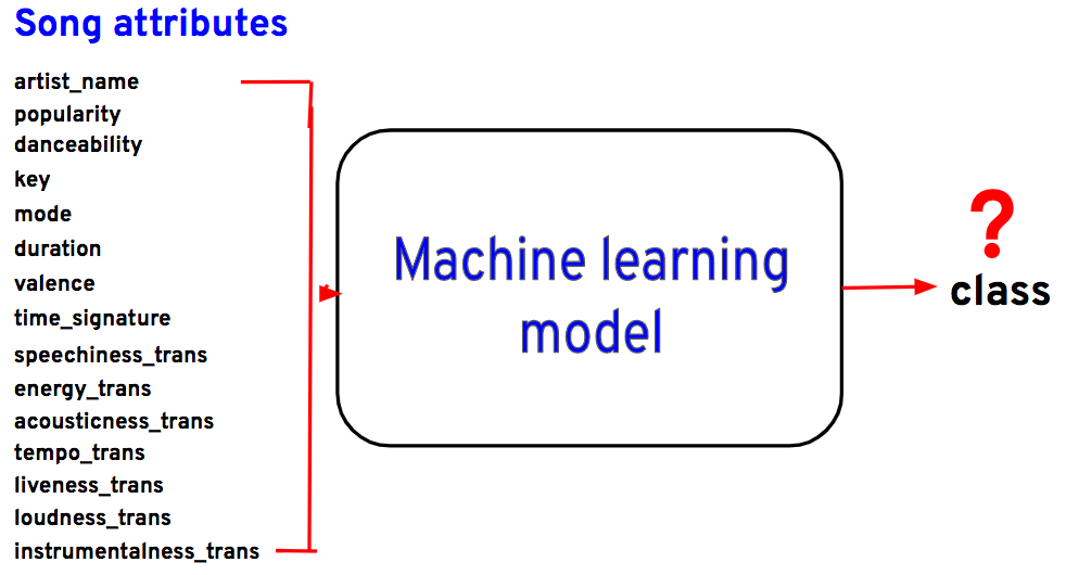
Steps to build music genre classification model

Classifying music genres used to be a complicated and time-consuming process, but machine learning has made it possible to do the task in a matter of seconds. So let's take a look at the steps required to create a machine learning model that classifies music.

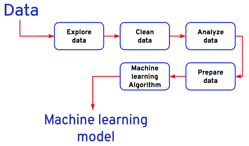
Required libraries

1. To explore, clean, and analyze data, we’ll use the Python libraries Pandas,** Numpy**, Matplotlib, and Seaborn.
2. To prepare data (feature engineering), to build models, to evaluate models, and to do hyperparameter tuning, we use Python’s machine learning library called Scikit-learn or sklearn.

We’ll import these libraries as and when needed.

Explore data

Image description

For this use case we’ll use a public dataset from Kaggle.

1. Import libraries
2. Load the dataset
3. How many records and variables are there in the given dataset and what are the data types of variables?
4. Meta data (brief explanation of all the variables)
   What’s the target variable? Is it categorical or quantitative? 5. If the target variable is categorical, check the number of categories in the target features.
5. What are the input or predictor variables?

1. Import libraries

1 import pandas as pd # import pandas library
2 import numpy as np # import numpy library
3 import matplotlib.pyplot as plt # import matplotlib library
4 import seaborn as sns # import seaborn library

2. Load the dataset using Pandas library and store it in a variable for easy access.

1 df = pd.read_csv("/content/music_data.csv")
2 df

3. How many records and variables are there in the given dataset and what are the data types of variables?

We’ll use the info() function to check the number of records, variables, and data types of variables in the given dataset.

1 df.info()

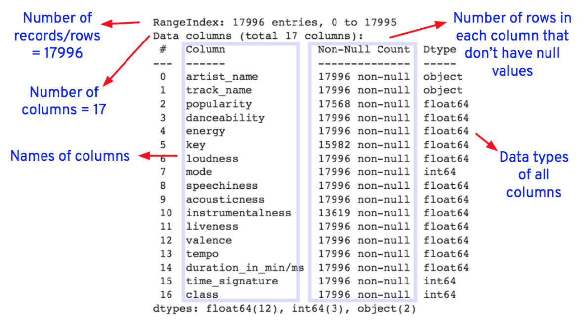
Why is it important to understand the shape and data types of a dataset?

• Rows: If there are too many rows, the algorithm takes too long to train, and if there are too few rows, the data may not be sufficient to produce good results.

• Columns or features: If the model has too many features (i.e., features equal to the number of rows), it may perform poorly.

• Data types: Understanding data types is important because it's possible that the data types of features are incorrect (i.e., numerical data saved in string format, etc.). In addition, if there are any categorical features, they must be converted into numerical data before being fed into a machine learning algorithm.

4. Meta data
Why is it important to understand metadata?
Metadata provides explicit information about what each column represents. This data helps us identify redundant features in the dataset.

5. What’s the target variable? Is it categorical or quantitative? If the target variable is categorical, check the number of categories in the target features.
"class" column is the target variable, as our goal is to classify the genre of a given song, and it’s a categorical variable. There are 11 categories in the "class" column.

6. What are the input or predictor variables?
Except for the “class” column, all the remaining columns are predictor variables or input variables.

Image description

1. Edit column names
2. Remove duplicate rows

1. Edit column names
Convert column names into lowercase letters and replace white spaces with an underscore (_). The column names are strings, so we use Python’s in-built functions str.lower() method to convert uppercase letters to lowercase and str.replace() method to replace white spaces with an underscore.

1 print("Original column names = ", df.columns)
2
3 df.columns= df.columns.str.replace(" ","_").str.lower()
4 print("Column names after conversion = ", df.columns)

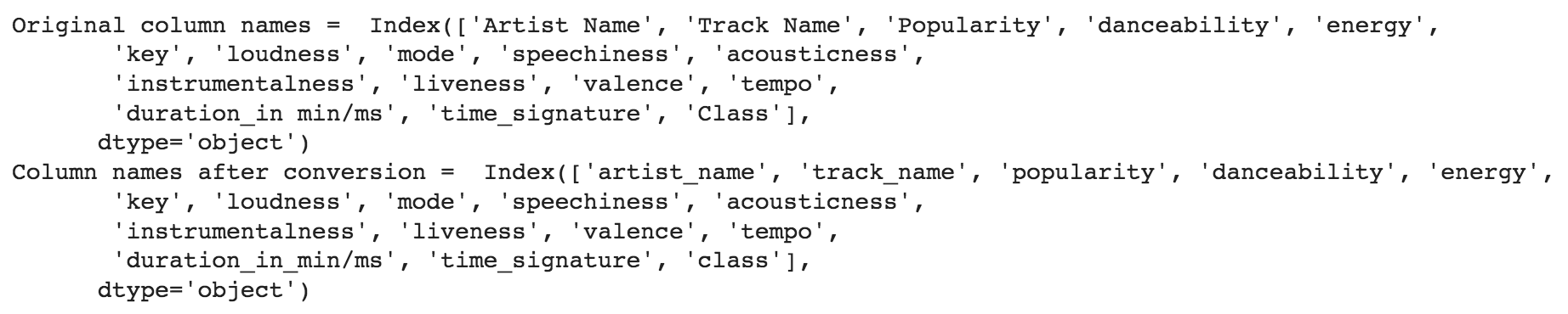
• Change column values: Let's look at the "duration in min/ms" column in more detail. Some values are in minutes, while others are in milliseconds. So, change all of the values in this column to milliseconds and rename it "duration in ms."

• Filter all the rows that have "duration" in minutes using the Pandas loc() method. Learn more about filtering operations in this article.

1 # Filter all the rows that have duration value less than "30"
2 df.loc[(df['duration_in_min/ms'] < 30)]['duration_in_min/ms']

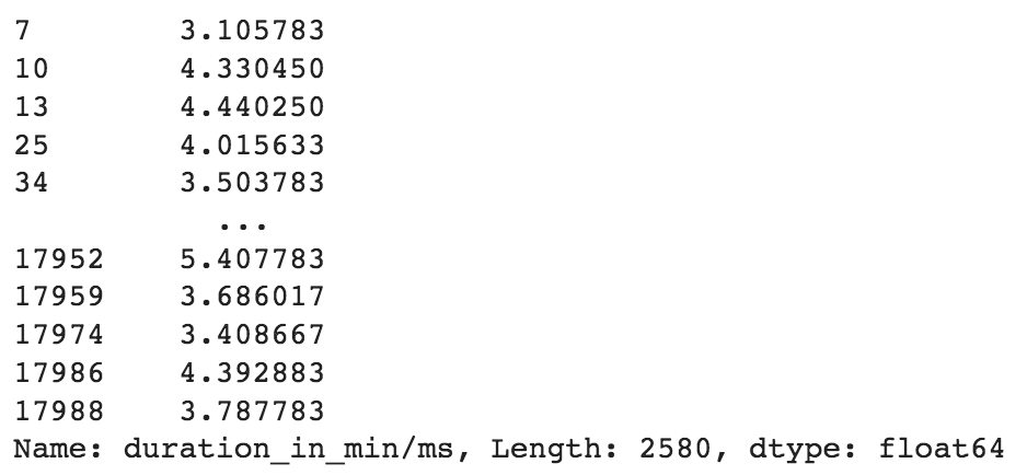Rows that have duration values in minutes

There are 2580 rows that have duration values in minutes. Let’s convert these values into milliseconds.

• Convert the values into milliseconds: 1 minute = 60,000ms, so let’s multiply the values in minutes by 60,000 and convert them into milliseconds.

1 condition = df['duration_in_min/ms'] < 30 
2
3 # If the value in duration_in_min/ms column is less than 30, then multiply the value with 60,000
4 df.loc[condition,'duration_in_min/ms'] = df.loc[condition,'duration_in_min/ms']*60000

• Rename the column “duration_in_min/ms” to “duration_in_ms” using Pandas rename() method.

1 df.rename(columns={"duration_in_min/ms": "duration_in_ms"})

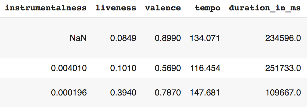Renamed duration_in_min/ms to duration_in_ms_

2. Are there duplicated rows or columns?

• Check for duplicate rows in the dataset with the duplicated() function. Except for the target variable, duplicate rows have the same values across all columns. So, we'll remove the target variable "class" from the dataset and look for duplicate rows.

1 duplicateRows = df[df.duplicated(subset = df.columns.difference(['class']))]

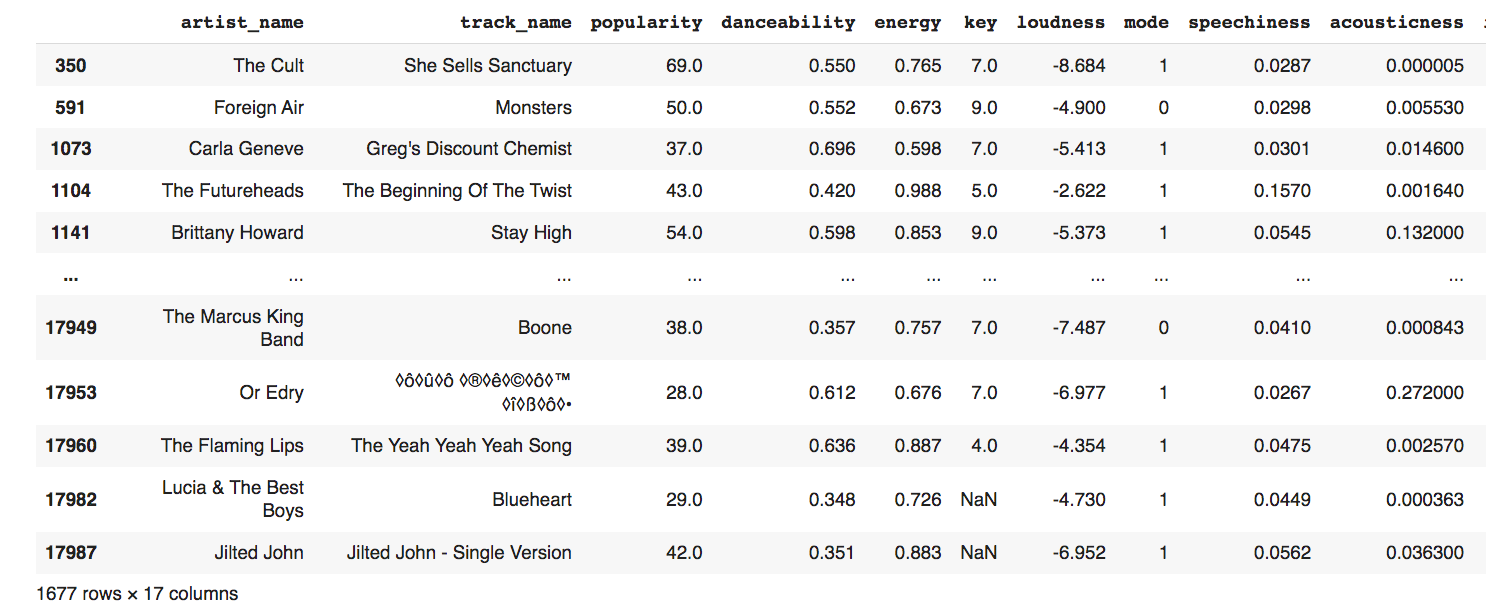Sample of duplicate rows_

There are 1677 duplicate rows that have the same values across all the columns. Refer this article to know more about duplicate values and how to remove them in detail.

• Using the drop_duplicates() function, delete the rows that have duplicate values across all columns.

1 print("Shape of dataset before removing duplicate rows =", df.shape)
2
3 df.drop_duplicates(subset = df.columns.difference(['class']), inplace = True, ignore_index = True)
4 print("Shape of dataset after removing duplicate rows =", df.shape)

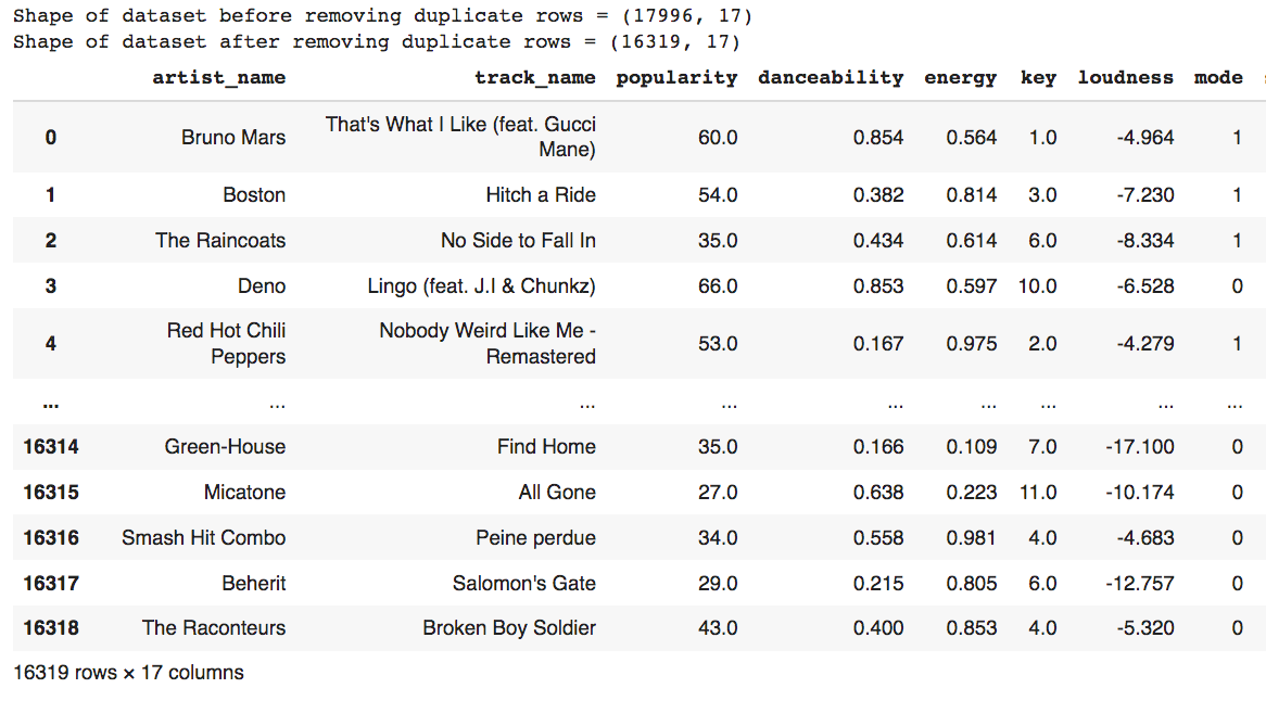Dataset after removing duplicate rows_

Analyze data

1. Are there null values?
2. What’s the data distribution of predictor variables? Is data skewed or normally distributed?
3. Are there outliers in the predictor or input variables?
4. How are the categories distributed in the target variable?
5. Is there a correlation between the input variables?

**1. Display the columns that have NaN values along with the count of NaN values. **
We’ll use the isnull() and any() functions to display the columns that have null values and the sum() function to calculate the total number of null values in the column.

1 nan_col = df.columns[df.isnull().any()]
2 for i in nan_col:
3    print(i, df[i].isnull().sum())

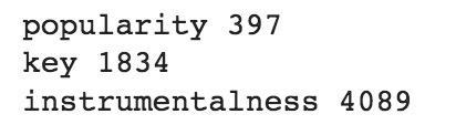
“popularity,” “key,” and “instrumentalness” columns have NaN values.

Why is it important to check for null values?
As the machine learning algorithms don't work for data with null or NaN values, it’s good to check for null values in the data. Learn more about missing or null values in this article.

2. What’s the data distribution of predictor variables? Is data skewed or normally distributed?

1 df_cont = df.select_dtypes([int,float]) # store all integer or float columns in df_cont variable
2
3 fig = plt.figure(figsize=(15, 18)) # sets the size of the 4 plot with width as 15 and height as 18
4 for i,columns in enumerate(df_cont.columns, 1): 
5    ax = plt.subplot(5,3,i) # creates 3 subplots in one single row
6    sns.kdeplot(x=df_cont[columns]) # creates kde plots for each feature in df_cont dataset
7    ax.set_xlabel(None) # removes the labels on x-axis
8    ax.set_title(f'Distribution of {columns}') # adds a title to each subplot
9    plt.tight_layout(w_pad=3) # adds padding between the subplots
10 plt.show() # displays the plots

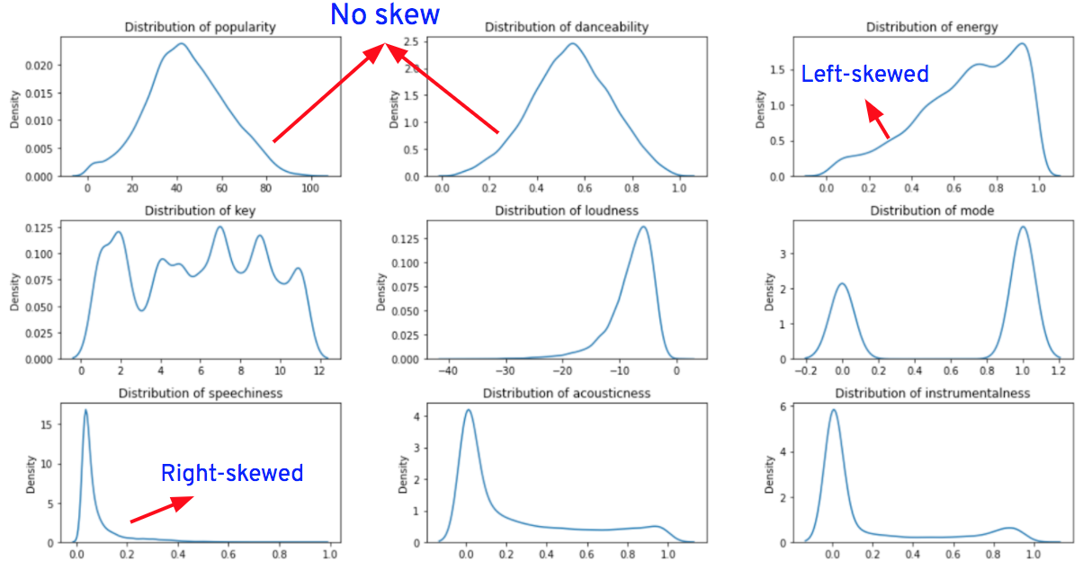
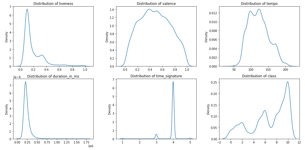
The skew() function in the Pandas library is used to determine the amount of skewness in each column.

1 df_cont = df.select_dtypes([int,float]) # store all integer or float columns in df_cont variable
2
3 for i in df_cont.columns:
4   print(f'Skewness in {i} =',df_cont[i].skew())

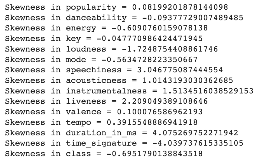
If skewness is in between -0.5 and 0.5, the data is more or less normally distributed, otherwise the data is skewed. So, from the skewness table, we can say that except for the "popularity," "danceability" and "valence" columns, all the other column distributions are either left-skewed or right-skewed.
Note: Columns "class," "mode," and "key" are of categorical data type. As their values are in numerical format, they're identified as integer columns and hence their distributions are plotted. So, we can ignore these columns while analyzing the distributions.

Why is it important to understand the distribution of features?
Some algorithms work best if the data is normally distributed. So, it’s always recommended to check for the skewed distributions and transform them into normally distributed features (close to normal distribution) before feeding them into a machine learning algorithm. Learn more about distributions in this article.

3. Are there outliers in the input variables?

1 df_cont = df.select_dtypes([int,float]) # store all integer or float columns in df_cont variable
2
3 fig = plt.figure(figsize=(10, 10)) # sets the size of the 4 plot with width as 10 and height as 10
4 for i,columns in enumerate(df_cont.columns, 1): 
5    ax = plt.subplot(5,3,i) # creates 3 subplots in one single row
6    sns.boxplot(data = df_cont, x=df_cont[columns]) # creates box plots for each feature in df_cont dataset
7    ax.set_xlabel(None) # removes the labels on x-axis
8    ax.set_title(f'Distribution of {columns}') # adds a title to each subplot
9    plt.tight_layout(w_pad=3) # adds padding between the subplots
10 plt.show() # displays the plots

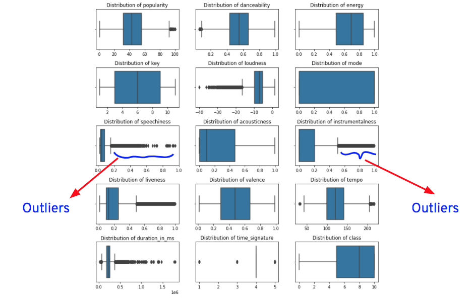
Outliers are represented as dots after the vertical lines on either side of the boxes. Except for "energy," "key," "acousticness," and "valence" columns, all the other columns have outliers.

Note: We’ll not consider "class," "mode," and "key" columns while looking for outliers, as they’re categorical columns that have values in number format.

Why is it important to check for outliers in a dataset?
Outliers affect the machine learning model’s performance. So, it’s important to check for outliers and treat them before feeding the data into an algorithm.

4. How are the categories distributed in the target variable?
We’ll use the countplot() function from the seaborn library to plot the distribution of categories in the target variable.

1 sns.countplot(data = df, x= df["class"])
2 plt.show()

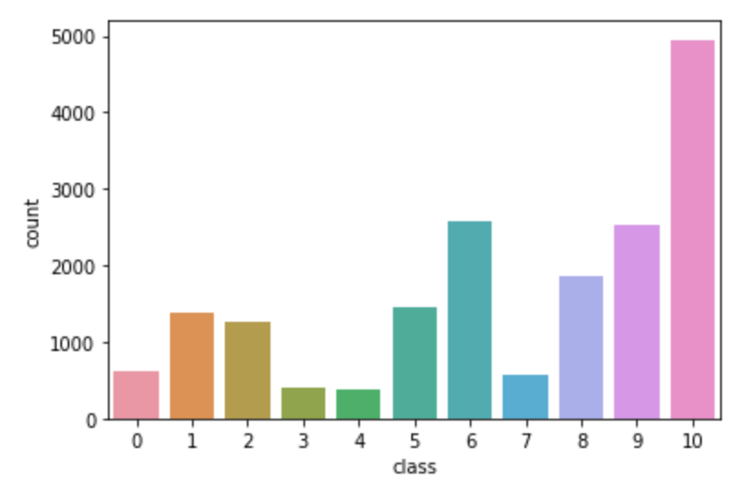
The distribution of classes looks almost balanced. There are nearly 5000 records with the label "class 10" and the rest of the classes have nearly 3000 or less than 3000 records. So, we can use it as it is, but if the machine learning model’s performance is not good, then we can come back and add synthetic data to make the data more balanced.

Why is it important to check the distribution of categories?
If the categories are imbalanced, then the obtained machine learning model may be biased. To avoid bias, we need to balance the categories by adding synthetic data. Learn more about the distribution of categories in this article.

5. Is there a correlation between the input variables?
The following correlation map displays the correlation between all the numerical (int or float data type) columns.

• A correlation value of +1 indicates that there is a strong positive correlation between the columns.
• A correlation value of -1 indicates that there is a strong negative correlation between the columns.
• A correlation value of 0 indicates that no correlation exists between the columns.

We remove 1 of the columns from the dataset that shows a positive or negative correlation.

The corr() function from the Pandas library calculates the correlation between the variables, and the heatmap() function from the Seaborn library plots the values in the form of a graph.

1 df_cont = df.select_dtypes([int,float]) # store all integer or float columns in df_cont variable
2
3 plt.figure(figsize=(16, 6)) # set the output figure size
4 sns.heatmap(data = df_cont.corr(), vmin = -1, vmax = 1, annot = True) 

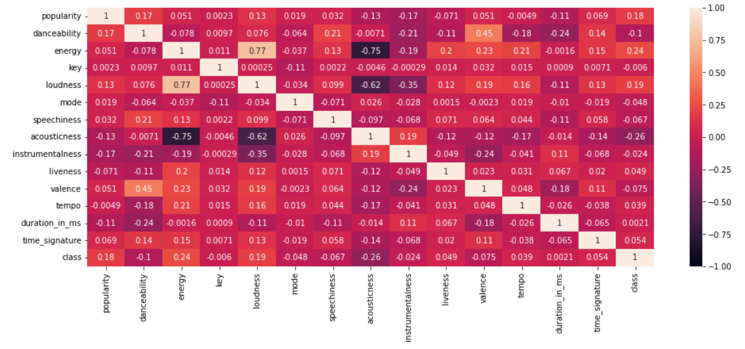
From the map, we see that

• “energy” and “loudness” show a positive correlation (0.77).
• “energy” and “acousticness” show a negative correlation (-0.75).
• “loudness” and “acousticness” show a negative correlation (-0.62).

1. Fill null or NaN values
2. Remove features that are highly correlated
3. Handle skewness
4. Treat outliers
5. Categorical data encoding

1. Fill null or NaN values
The following are the 3 columns that have null values

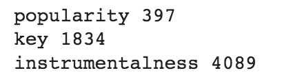
Let’s take a look at metadata of these columns

Based on the above information, we can fill or impute the missing values in each column in the following way.

• popularity and instrumentalness: NaN values in these columns can be filled with the mean or median value of their respective columns. When we plotted boxplots, we've seen that these 2 columns have outliers.

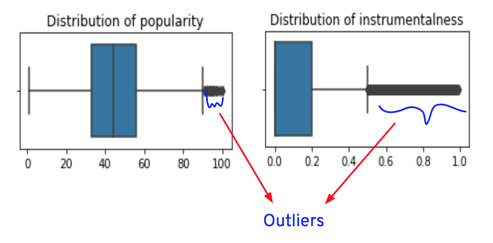
So, it’s suggestable to fill the NaN values with the median value of their respective columns.

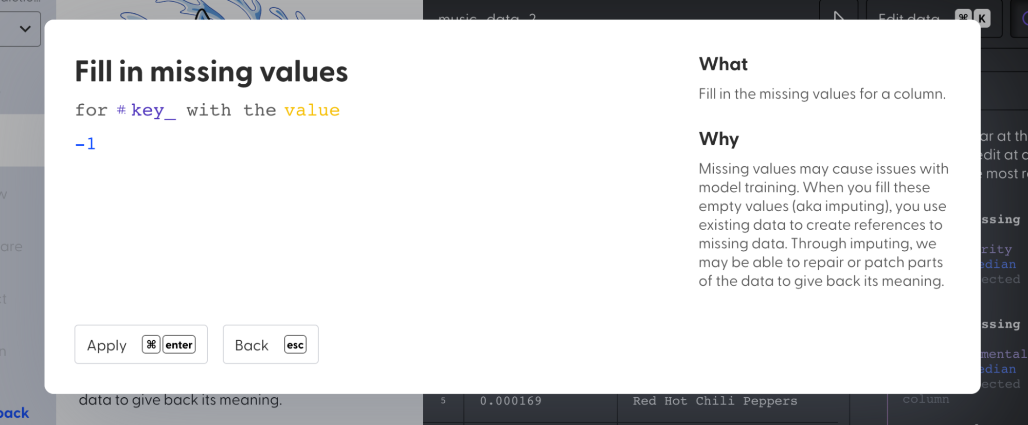
• key: It’s already mentioned in the information provided that if no key was detected, the value is -1. So, let’s fill the NaN values in this column with -1.

Imputation
Imputation means filling NaN values with guesstimate values. There are many ways to impute missing or NaN values. Check this article to learn more about imputation and the various imputation techniques available.

Impute null values in the "popularity" and "instrumentalness" columns with the median value. We’ll utilize the SimpleImputer class from Scikit-learn to impute null or NaN values.

1 from sklearn.impute import SimpleImputer
2 imp = SimpleImputer(missing_values = np.nan, strategy = 'median')
3 df[['popularity','instrumentalness']] = imp.fit_transform(df[['popularity','instrumentalness']])

1 df[['popularity','instrumentalness']].isnull().sum()

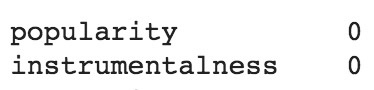
• Impute null values in the “key” column with a constant value -1.

1 from sklearn.impute import SimpleImputer
2 imp = SimpleImputer(missing_values=np.nan, strategy='constant', fill_value = -1)
3 df[['key']]=imp.fit_transform(df[['key']])

1 print("Count of null values in 'key' column =",df['key'].isnull().sum())

2. Remove features that are highly correlated

• "energy" and "loudness" show a positive correlation (0.77).
• "energy" and "acousticness" show a negative correlation (-0.75).
• "loudness" and "acousticness" show a negative correlation (-0.62).

Based on these observations, we can conclude that the "energy" column is highly correlated with the "acousticness" and "loudness" columns. So, we can remove the "energy" column from the dataset as it’s a redundant feature.

Drop the "energy" column from the dataset using the Pandas library drop() method.

3. Handle skewness
We can either minimize or remove skewness by using one of the transformation techniques like square root, cube root, reciprocal, square, or cube. We’ll apply all the techniques and then visualize the distributions of transformed columns or features. We’ll finally choose 1 technique that has transformed the column’s distribution close to a normal distribution and replace the original column values with the transformed column values.

We use Python’s Numpy library to apply these transformation techniques to the skewed data.

After applying the transformations for the columns "duration_in_ms," "loudness," "speechiness," "acousticness," "instrumentalness," "liveness," and "tempo," the data distributions of these columns are as shown below.

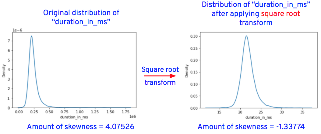
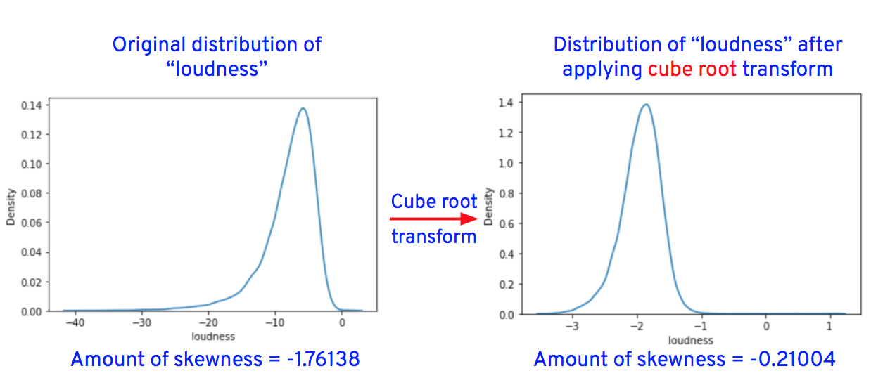
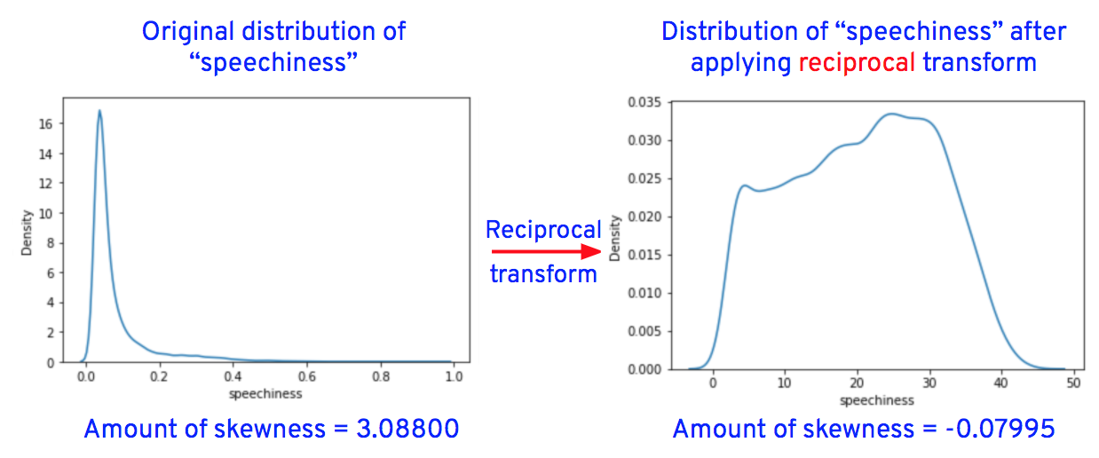
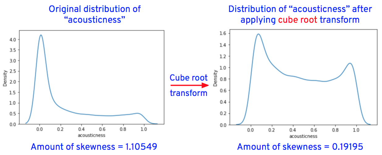
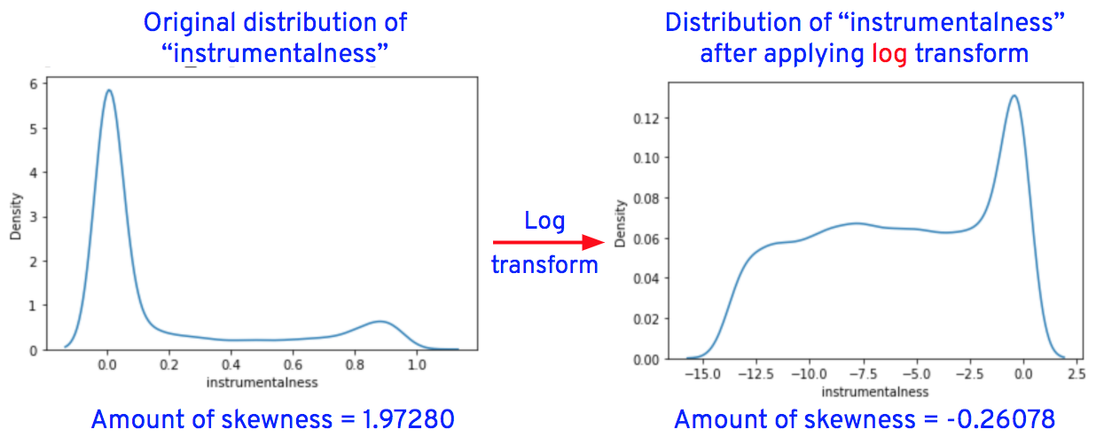
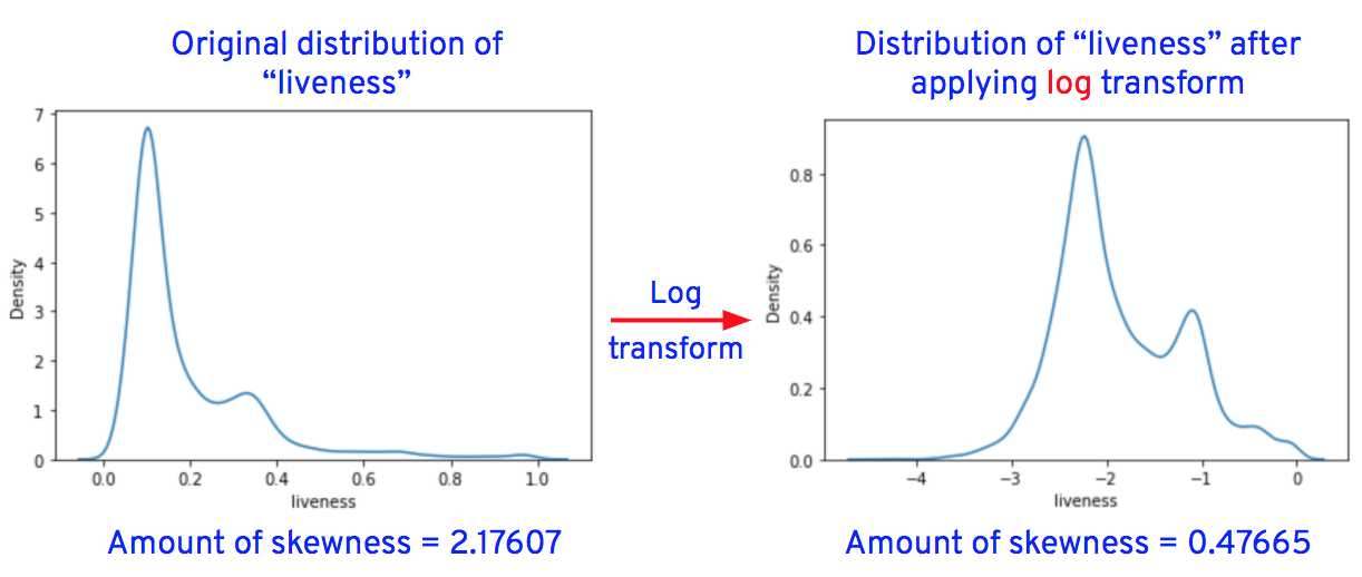
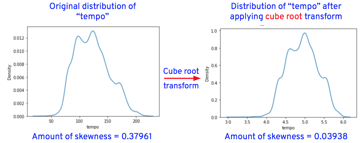
Now let’s replace the original column values of “loudness,” “speechiness,” “acousticness,” “instrumentalness,” “liveness,” and “tempo” with transformed values.

Replace "loudness" column values with the cube root of "loudness" column values, for example, if the original value of "loudness" is 8, the transformed value is 2 (i.e., the cube root of 8 = 2).

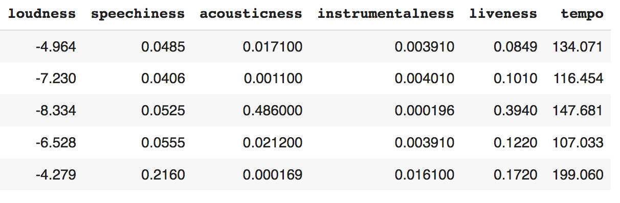
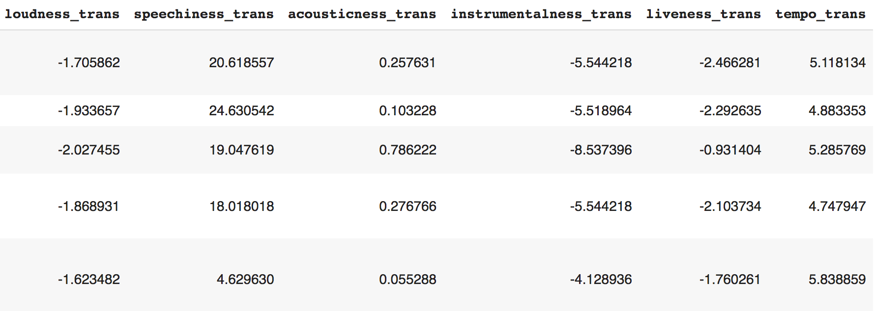
4. Remove outliers
Some of the techniques used to remove outliers are:

1. Transforming columns by using transformation techniques such as log, exponential, reciprocal, square root, etc., removes outliers.
2. Replace outliers with either an upper or lower limit value. These upper and lower limit values are calculated using a statistical method called IQR.
3. Replace the outliers with the mean, median, or mode value of the column.
4. Delete rows from the dataset that have outliers. (This technique is used rarely.

Choosing a technique to treat outliers is a hit and trial process. Depending on the model's performance, we’ll change the technique. For example, let’s say we replaced outliers with upper and lower limit values and assume this data is used to build a model. If the model’s performance is bad, then we’ll replace the outliers by using another technique and evaluate the model’s performance again. The process is repeated until the model performs well.

While transforming the columns to remove skewness, outliers will also be reduced as the same transformation techniques, such as log, cube root, etc., are used for treating outliers as well. So let’s plot the graphs and check for outliers in the transformed columns.

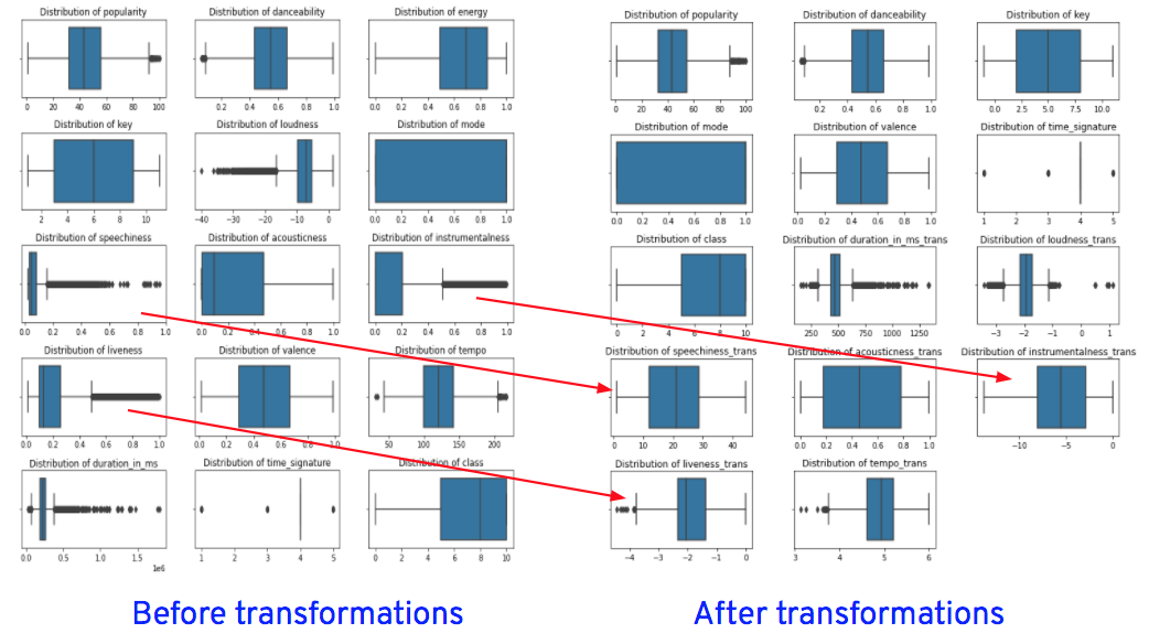
From the graphs, we see that the outliers in “speechiness” and “instrumentalness” are completely removed after transformations, while outliers in “loudness,” “liveness” and “tempo” are reduced after transformations.

5. Categorical data encoding
Machine learning algorithms understand only numbers, so before training the data, we’ll convert strings into numbers without losing any information. Encoding string data into numerical data is a hit-and-trial process. Choose any 1 of the techniques: convert the data, train the data, evaluate the model. If model performance results aren’t satisfactory, change the technique and repeat the process until you get the desired results.
We’ve 2 string columns in our dataset, "artist name" and "track name," that must be converted to numerical format.
Some techniques that are used to convert string data into numerical data are label encoding, ordinary encoding, one-hot encoding, frequency encoding, etc.
Let's try the label encoding technique to convert the "track_name" and "artist_name" columns into numeric data. We’ll use the LabelEncoder() class from Scikit-learn to perform this operation.

1 from sklearn.preprocessing import LabelEncoder
2 columns = ["artist_name","track_name"]
3 le = LabelEncoder()
4 for col in columns:
5   df[col] = le.fit_transform(df[col])

1 df[["artist_name","track_name"]]

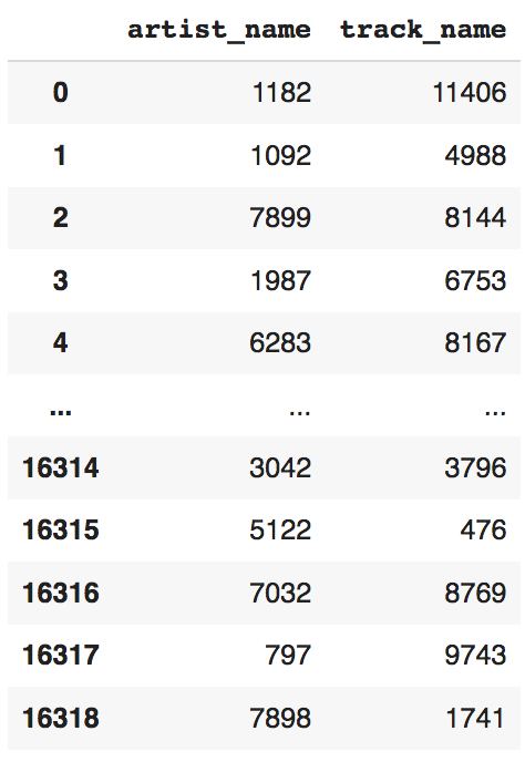“artist_name” and “track_name” columns after transformation_

Build machine learning model

Until now, we’ve seen how to explore, analyze, and prepare data to train the machine learning algorithms. Now it’s time to train the data using various machine learning algorithms and build machine learning models.

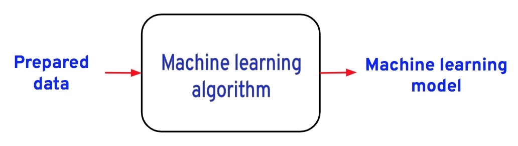
We’ll use Python’s machine learning library called Scikit-learn to train data and to build machine learning models.

1. Create 2 new variables (X and y), store all the predictor variables or inputs in X and the target variable “class” in y.

1 X = df.drop(columns=["class"], axis=1)
2 y = df["class"]

2. Split the dataset into training and test sets using Scikit-learn train_test_split method. We’re splitting the data in such a way that the train dataset is 67% and the test dataset is 33%(size = 0.33).

1 from sklearn.model_selection import train_test_split
2
3 X_train, X_test, y_train, y_test = train_test_split(X, y, test_size=0.33, random_state=11)

3. Standardize or normalize data: This is a feature engineering technique that helps to change the scale of the entire dataset into 1 format. This operation is performed only after splitting the dataset into training and test sets. The main reason to perform this operation after splitting the data is to avoid data leakage. We’ll use either StandardScaler(to standardize) or MinMaxScaler(to normalize) classes from the Scikit-learn library to change the scale of the dataset.

1 from sklearn.preprocessing import StandardScaler
2 scaler = StandardScaler()
3
4 normalized_x_train = pd.DataFrame(scaler.fit_transform(X_train), columns = X_train.columns)

Standardization

1 from sklearn.preprocessing import MinMaxScaler
2 scaler = MinMaxScaler()
3
4 normalized_x_train = pd.DataFrame(scaler.fit_transform(X_train), columns = X_train.columns)

Normalization

4. Train data using various machine learning algorithms and build models: Let’s train the prepared data using Logistic regression, decision tree classifier and random forest classifier algorithms.
   a. Logistic regression

1 from sklearn.linear_model import LogisticRegression
2 from sklearn.metrics import accuracy_score
3
4 LR = LogisticRegression(solver='liblinear').fit(normalized_x_train, y_train)
4 normalized_x_test = pd.DataFrame(scaler.transform(X_test), columns = X_test.columns)
6 y_pred = LR.predict(normalized_x_test)
7
8 LRAcc = accuracy_score(y_pred,y_test) # Calculate accuracy
9 print('Logistic Regression accuracy is: {:.2f}%'.format(LRAcc*100))

b. Decision tree classifier

1 from sklearn.tree import DecisionTreeClassifier
2 from sklearn.metrics import accuracy_score
3
4 DTclassifier = DecisionTreeClassifier(max_leaf_nodes=20).fit(normalized_x_train, y_train)
5 y_pred = DTclassifier.predict(normalized_x_test)
6
7 DTAcc = accuracy_score(y_pred,y_test) # Calculating accuracy
8 print('Decision Tree accuracy is: {:.2f}%'.format(DTAcc*100))

c. Random forest classifier

1 from sklearn.tree import DecisionTreeClassifier
2 from sklearn.metrics import accuracy_score
3
4 DTclassifier = DecisionTreeClassifier(max_leaf_nodes=20).fit(normalized_x_train, y_train)
5 y_pred = DTclassifier.predict(normalized_x_test)
6
7 DTAcc = accuracy_score(y_pred,y_test) # Calculating accuracy
8 print('Decision Tree accuracy is: {:.2f}%'.format(DTAcc*100))

Logistic regression performed well and gave us better accuracy than decision trees and random forest classifiers. To further improve accuracy, we can perform other operations like hyperparameter tuning, gathering more data, or better preparing the data.

Magical no code solution

As you’ve seen, building a machine learning model from scratch is a tedious and time-consuming process. Try our product Mage to build models within minutes. All the major steps, like feature engineering, model building, hyperparameter tuning, and evaluating the model are all handled by Mage. Your task is to just load the data, clean the data (Mage will give you a good number of suggestions to clean the data), manipulate columns, impute missing values and that's it. Once the data is cleaned, you can immediately start the training process, where it handles all the remaining steps and delivers you a machine learning model along with performance metrics, statistics, and many more just like that.

Data cleaning and Feature engineering using Mage:

• Convert duration values that are in minutes into milliseconds.
  Steps:

1. Click on “Edit data”
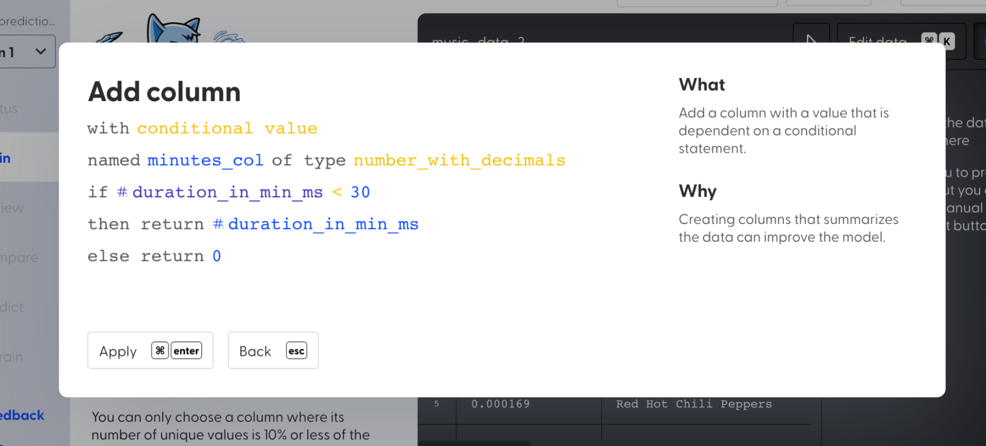
2. Select “Add column” transformer action and create a new column “minutes_col” with a condition such that the values are 0 if the “duration_in_min_ms” values are greater than 30 else return the “duration_in_min_ms” value.

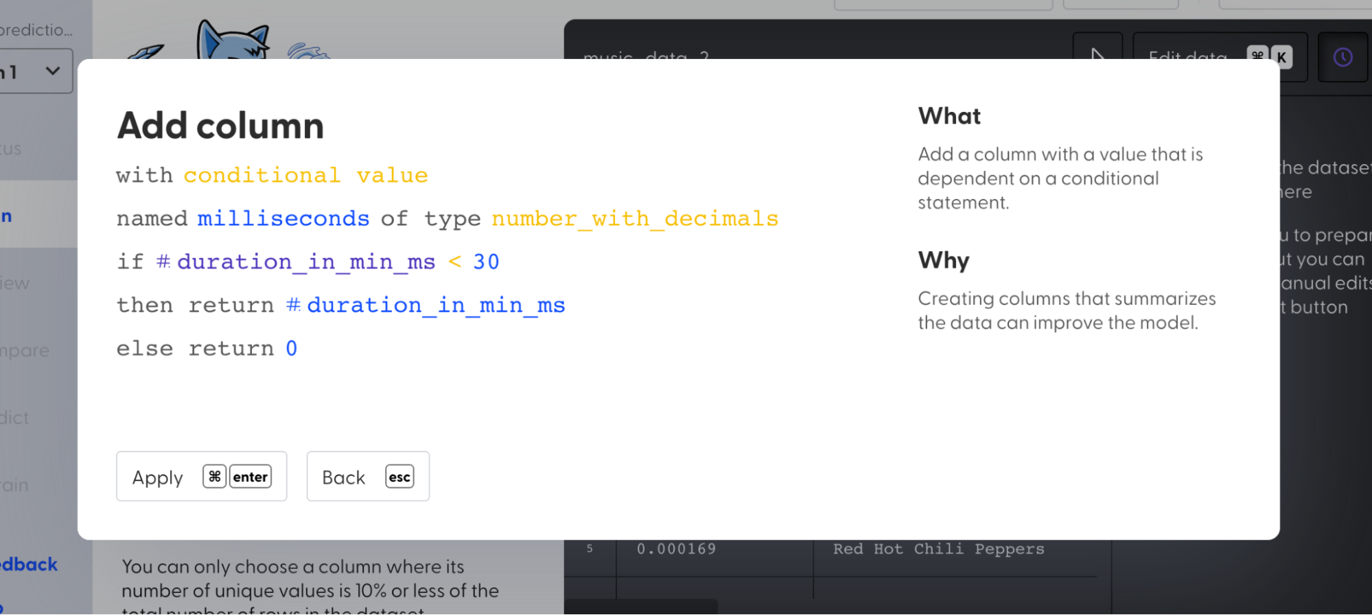
3. Select “Add column” and create a new column “milliseconds_col” with a condition such that the values are 0 if the “duration_in_min_ms” values are less than 30 else return the “duration_in_min_ms” value.

4. Select “Add column” and create a new column “min_to_ms” and multiply all the values in “minutes_col” with 60000.

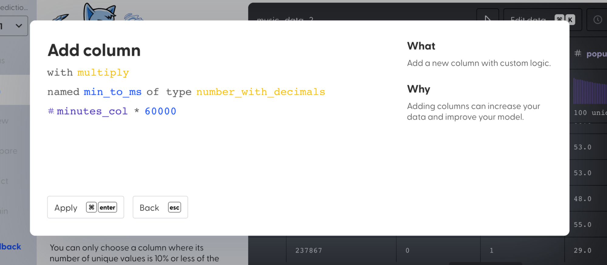
5. Select “Add column” and create a new column “duration” and sum all the values in “milliseconds_col” and “min_to_ms”.

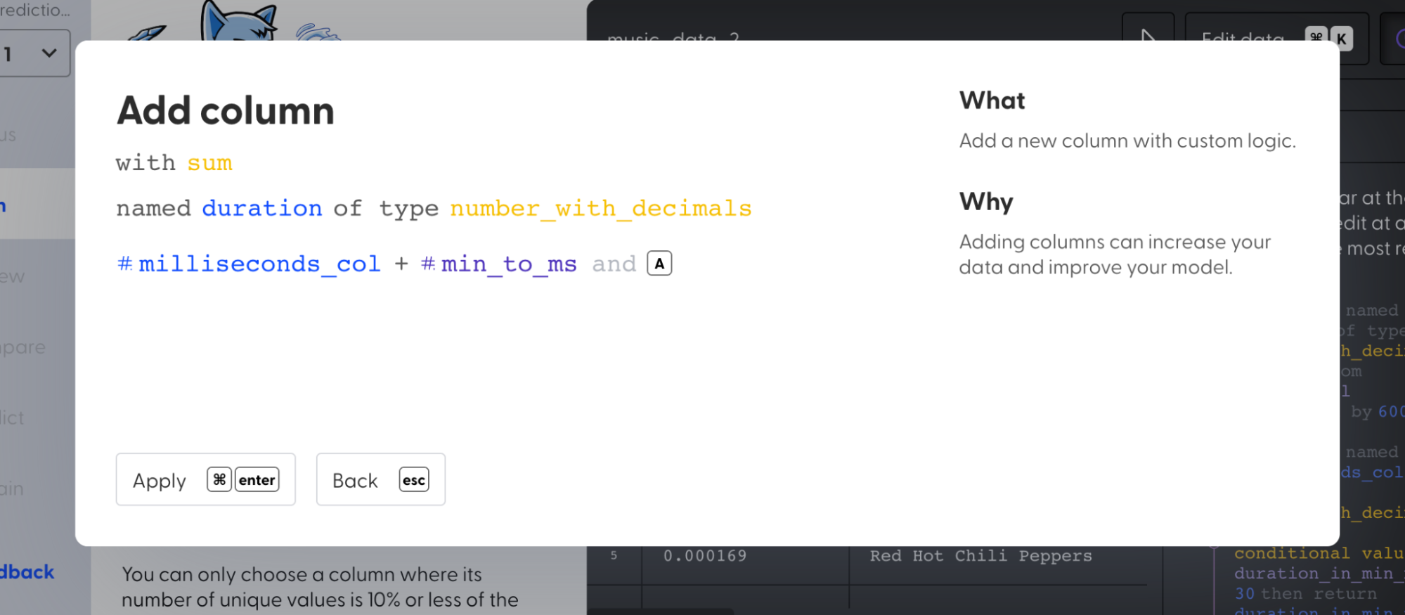
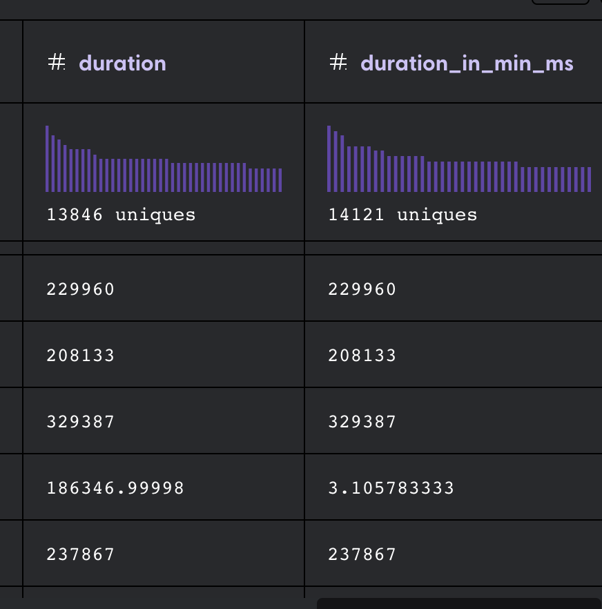
6. Now all the values in the “duration” column have been transformed to milliseconds.

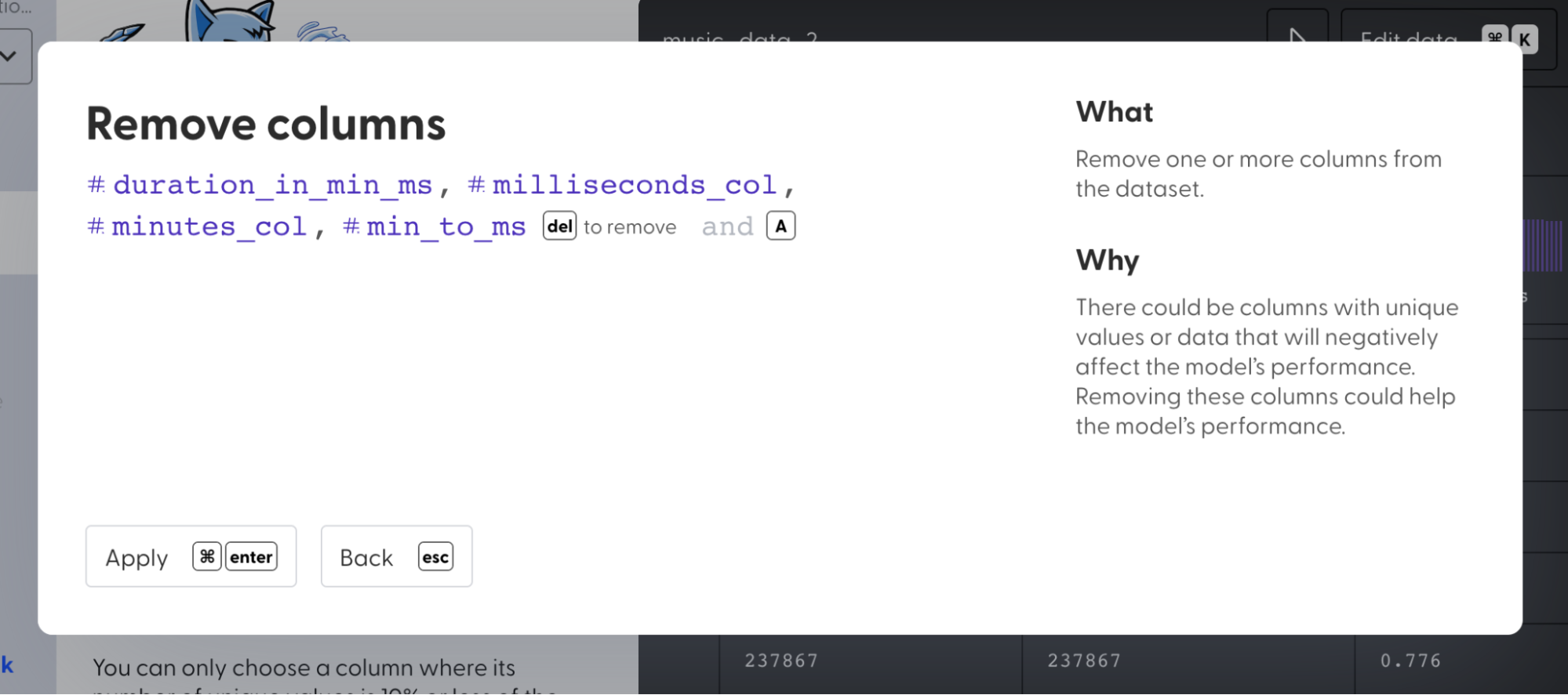
7. Select “Remove columns” and delete “duration_in_min_ms,” “minutes_col,” “milliseconds_col,” “min_to_ms” columns from the dataset as they’re redundant features.

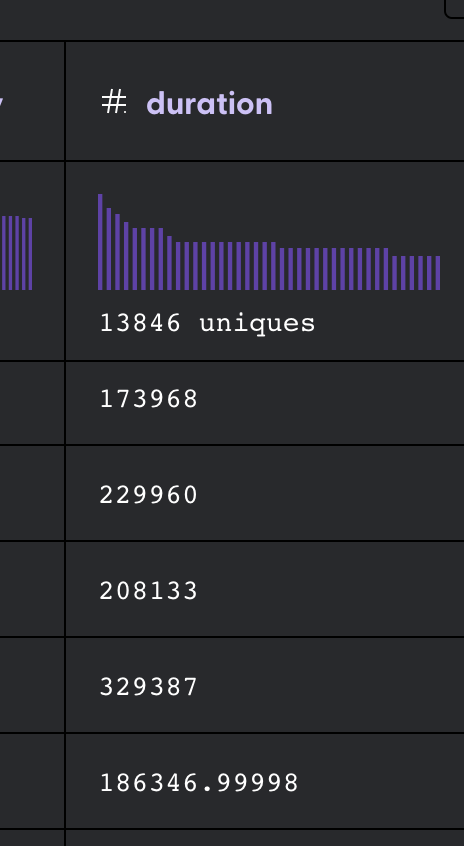Transformed column_

• Impute null or NAN values
  Steps:

1. Click on Edit data
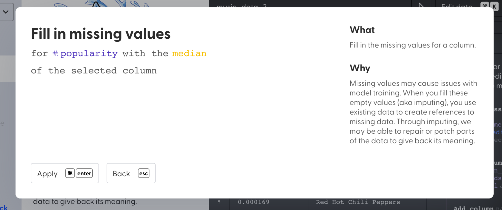
2. Select “Fill in missing values”
3. Fill the null values in columns “popularity” and “instrumentalness” with median value.

4. Fill the null values in the “key” column with a constant value -1

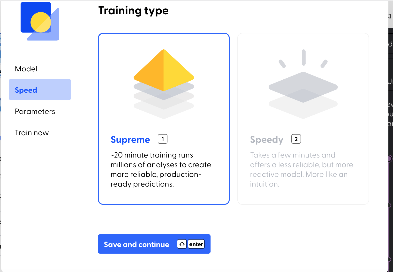
Build model using Mage: Once the data is ready, click on “Start training”

Next, click on ”Assign a new name to the model”>”Select Speed (Supreme)”

Finally, click on “Begin training” and see the magic happens.

During training_

Once the model training is completed, the user is provided with an overview of model performance, statistics, information about top features, etc.

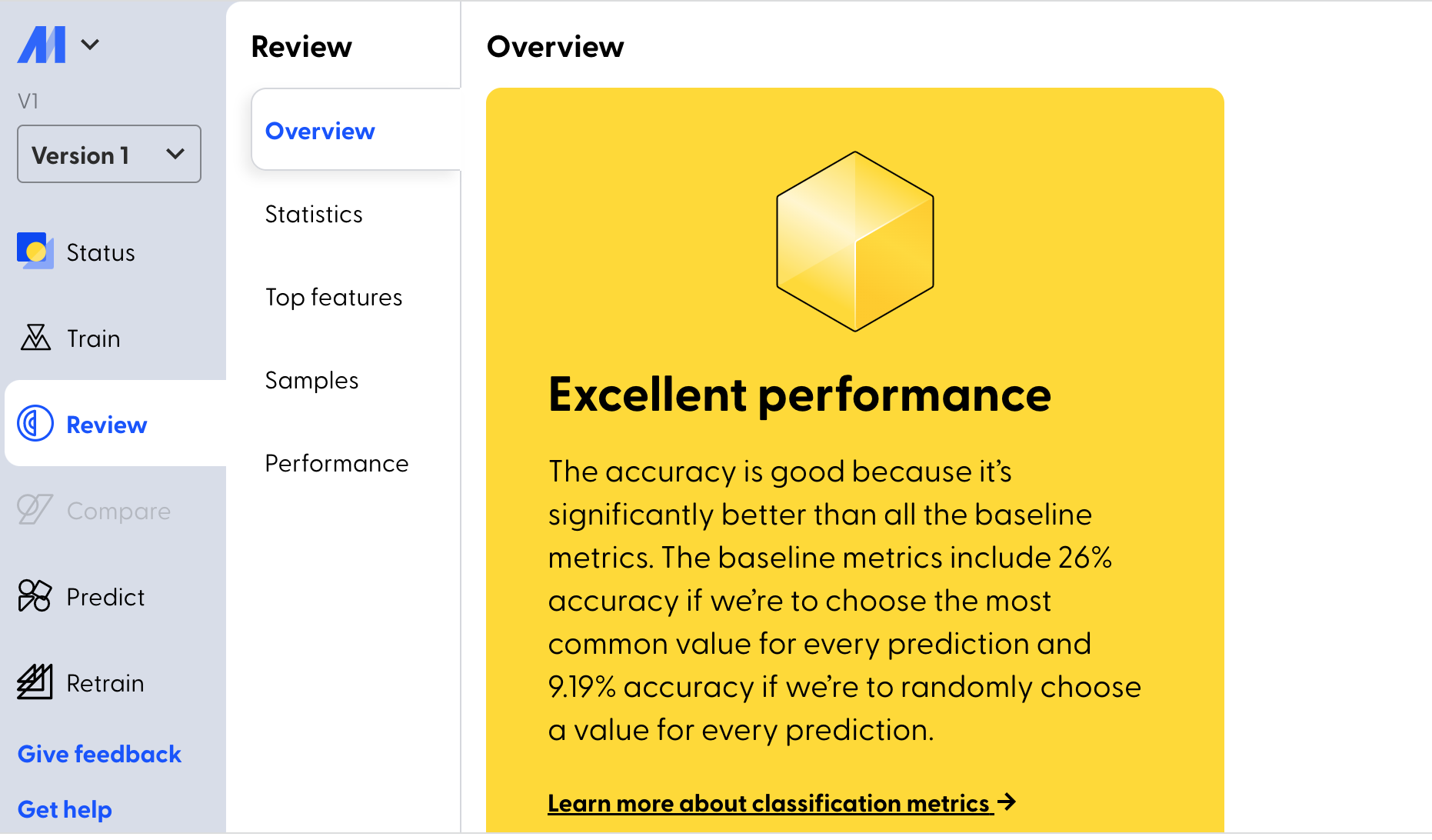
As you can see Mage gives you amazing results in less time and with less data preparation.
Note: If you wish to improve your model performance, Mage has a “Retrain” option to add or remove data or by following all the guided suggestions provided by Mage.